Quantization

원문 출처

 

• 양자화는 연속 데이터를 이산 숫자로 변환하는 과정이다.
• 신경망 훈련 계산은 일반적으로 Floating point type (16bit, 32bit)를 사용하여 수행된다.
• 딥러닝에서 양자화는 일반적으로 부동 소수점에서 고정 소수점 정수로 변환하는 것을 말한다.
• 딥러닝에서 사용되는 양자화 기술은 Dynamic Quantization, Static Quantization 등이 존재한다.

 

---

Quantization Mapping

• 양자화는 부동 소수점 값 \(x ∈ [ \alpha, \beta ]\)를 b-bit 정수 \(x_q ∈ [\alpha_q, \beta_q]\)에 맵핑한다.

de-Quantization 프로세스 수학적 정의

$$ x = c(x_q + d) $$

Quantization 프로세스 수학적 정의

$$ x_q = round(\frac{1}{c} x - d) $$

 

c, d : 변수(variables)

 

c 및 d를 유도하기 위하여 α가 αq에 대한 맵과 β가 βq 맵에 대한 맵을 확인하야하고, 선형 시스템 문제를 해결해야 한다.

 

\(\beta = c(\beta_q+d)\)

\(\alpha= c(\alpha_q+d)\)

 

솔루션은 다음과 같다.

\(c = \frac{\beta-\alpha}{\beta_q - \alpha_q}\)

\(d = \frac{\alpha\beta_q-\beta\alpha_q}{\beta - \alpha}\)

 

실제로, 양자화 후 에러 없이 Floating point "0"이 정확하게 표현되도록 해야 한다.

 

수학적 증명 : 

\(x_q = round(\frac{1}{c}0 -d)\)

\(= round(-d)\)

\(= -round(d)\)

\(= -d　　　\)

 

위 수식의 의미는 아래와 같다

\(d = round(d)\)

\(　　　= round(\frac{\alpha\beta_q-\beta\alpha_q}{\beta-\alpha})\)

 

컨벤션에 의해서 c를 스케일 s로 , -d를 zero point z로 표시한다.

 

요약

• Quantization

$$ x = s(x_q -z) $$

• de-quantization

$$ x_q = round(\frac{1}{s}x +z) $$

• 스케일 's' , Zero point 'z'의 값

\(s = \frac{\beta-\alpha}{\beta_q - \alpha_q}\)

\(z = round(\frac{\beta\alpha_q - \alpha\beta_q}{\beta-\alpha})\)

 

'z'는 정수, 's'는 부동 소수점이다.   

  

Value Clipping

• 실제로, 양자화 과정은 \( [\alpha, \beta]\)의 범위를 벗어난 \(x\) 를 가질 가능성이 있으며, 양자화 된 값 \(x_q\) 또한 \( [\alpha, \beta]\)의 범위를 벗어난다. 
• Integer type이 INTb 및 \( (alpha_q, \beta_q) = (-2^{b-1}, 2^{b-1} -1) \) 또는 unsigned UINTb \( (\alpha_q, \beta_q) = (0,2^b -1)\) 인 경우
  유형 정밀도가 범위를 벗어난 값을 클리핑 한다.
• 구체적으로, 양자화 진행에서는 추가 클립 단계가 있다.

$$ x_q = clip (round(\frac{1}{s}x+z), \alpha_q,\beta_q) $$

 

여기서 \(clip(x,l,u)\) 함수는 다음과 같이 정의 된다.

$$ clip(x,l,u) = \begin{cases} l\quad if\;x<1\\ x\quad if\;l\leq x\leq u\\ u\quad if\;x>u \end{cases} $$

 

Affine Quantization Mapping

• 위에서 설명한 Quantization Mapping을 Affine Quantization Mapping이라고도 한다.

Scale Quantization Mapping

• 정수형이 INTb로 부호화되면 \((\alpha_q, \beta_q) \ = \ (-2^{b-1}|1, \ 2^{b-1} -1)\) 이고, \(z \ = \ 0\) 을 강제 한다.
• 수학적으로는 아래와 같다

\(\alpha_q \ = \ -\beta_q\)

\(round(\frac{\beta\alpha_q-\alpha\beta_q}{\beta-\alpha} \ = \ 0)\)

 

• 위 결과 \( \alpha = -\beta\)가 생성 된다.
• 따라서, 부동 소수점 범위인 \([\alpha, -\alpha]\) 와 정수 범위 \([\alpha_q - \beta_q]\) 사이에서 매핑된다.
• 0을 중심으로 정확히 대칭이기 때문에, Symmetric Quantization Mapping 이라고도 한다.
• Scale Quantization Mapping은 Affine Quantization Mapping의 특수한 경우일 뿐이고, 정수 범위에 사용되지 않는 비트가 존재한다.

요약 (Summary)

• Quantization function

$$ f_q(x,s,z) \ = \ clip(round(\frac{1}{s}x + z),\alpha_q,\beta_q)$$

• de-Quantization function

$$ f_d(x_q,s,z)\ = \ s(x_q -z)$$

---

Quantized Matrix Multiplication

: 추후 작성

 

---

Quantized Deep Learning Layers

• 딥러닝 모델에서는 행렬 곱셈 외에도 ReLU와 같은 비선형 활성화 계층과 배치 정규화 같은 특수 계층이 존재한다.
• 실제로 양자화 된 딥러닝 모델에서 이러한 계층을 어떻게 처리할 것인가가 가장 중요한 문제이다.

간단한 솔루션

• 양자화 된 입력 텐서를 레이어로 역 양자화 하고, 일반적인 부동 소수점 계산을 사용하여 출력 텐서를 양자화 하는 것.
• 모델에 이러한 계층이 몇개만 존재하거나, 계층을 양자화된 방식으로 처리하기 위한 특별한 구현이 없는 경우에 작동한다.

대부분 딥러닝 모델에서 계층의 수는 무시 할 수 없으며, 위와 같은 간단한 솔루션을 사용하면 추론이 느려질 가능성이 크다.

 

Quantized ReLU

• 활성화 함수 ReLU를 아래와 같이 정의한다.
• 기존 ReLU 정의와 다르지만, 더 일반화 되어 양자화 된 ReLU 구현에 편리하다.

$$ ReLU(x,z_x,z_y,k)\ = \ \begin{cases} z_y  \quad if \; x \leq z_x \\ z_y + k(x-z_x) \quad if \; x \geq z_x \end{cases} $$

 

• 딥러닝 모델에서 일반적으로 사용되는 ReLU는 \(z_x=0,\quad z_y=0, \quad k=1\)일 때 위 정의의 특수한 경우입니다.

$$ ReLU(x,0,0,1)\ = \ \begin{cases} 0  \quad if \; x \leq 0 \\ x \quad if \; x \geq 0 \end{cases} $$

 

• ReLU가 수학적으로 어떻게 양자화되었는지 증명해 보겠습니다.

출처 : Lei Mao Github

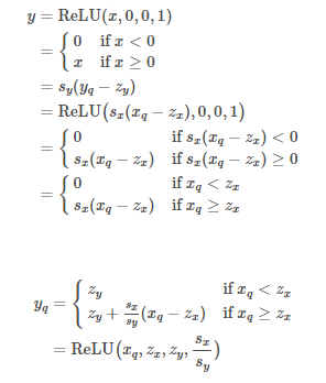
따라서 부동 소수점 \(y= ReLU(x,0,0,1)\)에 해당하는 양자화된 ReLU를 수행하려면 \(y_q=ReLU(x_q,z_x,z_y,\frac{s_x}{s_y})\)만 하면 된다.

 

양자화된 ReLU 레이어에 대한 소스 코드

import numpy as np


def quantization(x, s, z, alpha_q, beta_q):

    x_q = np.round(1 / s * x + z, decimals=0)
    x_q = np.clip(x_q, a_min=alpha_q, a_max=beta_q)

    return x_q


def quantization_int8(x, s, z):

    x_q = quantization(x, s, z, alpha_q=-128, beta_q=127)
    x_q = x_q.astype(np.int8)

    return x_q


def quantization_uint8(x, s, z):

    x_q = quantization(x, s, z, alpha_q=0, beta_q=255)
    x_q = x_q.astype(np.uint8)

    return x_q


def dequantization(x_q, s, z):

    # x_q - z might go outside the quantization range
    x_q = x_q.astype(np.int32)
    x = s * (x_q - z)
    x = x.astype(np.float32)

    return x


def generate_quantization_constants(alpha, beta, alpha_q, beta_q):

    # Affine quantization mapping
    s = (beta - alpha) / (beta_q - alpha_q)
    z = int((beta * alpha_q - alpha * beta_q) / (beta - alpha))

    return s, z


def generate_quantization_int8_constants(alpha, beta):

    b = 8
    alpha_q = -2**(b - 1)
    beta_q = 2**(b - 1) - 1

    s, z = generate_quantization_constants(alpha=alpha,
                                           beta=beta,
                                           alpha_q=alpha_q,
                                           beta_q=beta_q)

    return s, z


def generate_quantization_uint8_constants(alpha, beta):

    b = 8
    alpha_q = 0
    beta_q = 2**(b) - 1

    s, z = generate_quantization_constants(alpha=alpha,
                                           beta=beta,
                                           alpha_q=alpha_q,
                                           beta_q=beta_q)

    return s, z


def relu(x, z_x, z_y, k):

    x = np.clip(x, a_min=z_x, a_max=None)
    y = z_y + k * (x - z_x)

    return y


def quantization_relu_uint8(x_q, s_x, z_x, s_y, z_y):

    y = relu(x=x_q.astype(np.int32), z_x=z_x, z_y=z_y, k=s_x / s_y)
    y = np.round(y, decimals=0)
    y = np.clip(y, a_min=0, a_max=255)
    y = y.astype(np.uint8)

    return y


if __name__ == "__main__":

    # Set random seed for reproducibility
    random_seed = 0
    np.random.seed(random_seed)

    # Random matrices
    m = 2
    n = 4

    alpha_X = -60.0
    beta_X = 60.0
    s_X, z_X = generate_quantization_int8_constants(alpha=alpha_X, beta=beta_X)
    X = np.random.uniform(low=alpha_X, high=beta_X,
                          size=(m, n)).astype(np.float32)
    X_q = quantization_int8(x=X, s=s_X, z=z_X)
    X_q_dq = dequantization(x_q=X_q, s=s_X, z=z_X)

    alpha_Y = 0.0
    beta_Y = 200.0
    s_Y, z_Y = generate_quantization_uint8_constants(alpha=alpha_Y,
                                                     beta=beta_Y)
    Y_expected = relu(x=X, z_x=0, z_y=0, k=1)
    Y_q_expected = quantization_uint8(x=Y_expected, s=s_Y, z=z_Y)

    Y_expected_prime = relu(x=X_q_dq, z_x=0, z_y=0, k=1)
    Y_expected_prime_q = quantization_uint8(x=Y_expected_prime, s=s_Y, z=z_Y)
    Y_expected_prime_q_dq = dequantization(x_q=Y_expected_prime_q,
                                           s=s_Y,
                                           z=z_Y)

    print("X:")
    print(X)
    print("X_q:")
    print(X_q)

    print("Expected FP32 Y:")
    print(Y_expected)
    print("Expected FP32 Y Quantized:")
    print(Y_q_expected)

    Y_q_simulated = quantization_relu_uint8(x_q=X_q,
                                            s_x=s_X,
                                            z_x=z_X,
                                            s_y=s_Y,
                                            z_y=z_Y)
    Y_simulated = dequantization(x_q=Y_q_simulated, s=s_Y, z=z_Y)

    print("Expected Quantized Y_q from Quantized ReLU:")
    print(Y_q_simulated)
    print("Expected Quantized Y_q from Quantized ReLU Dequantized:")
    print(Y_simulated)

    # Ensure the algorithm implementation is correct
    assert (np.array_equal(Y_simulated, Y_expected_prime_q_dq))
    assert (np.array_equal(Y_q_simulated, Y_expected_prime_q))

• 결과 값

$ python relu.py 
X:
[[ 5.8576202 25.822723  12.331605   5.385982 ]
 [-9.161424  17.507294  -7.489535  47.01276  ]]
X_q:
[[ 12  55  26  11]
 [-19  37 -16 100]]
Expected FP32 Y:
[[ 5.8576202 25.822723  12.331605   5.385982 ]
 [ 0.        17.507294   0.        47.01276  ]]
Expected FP32 Y Quantized:
[[ 7 33 16  7]
 [ 0 22  0 60]]
Expected Quantized Y_q from Quantized ReLU:
[[ 7 33 16  7]
 [ 0 22  0 60]]
Expected Quantized Y_q from Quantized ReLU Dequantized:
[[ 5.490196 25.882353 12.54902   5.490196]
 [ 0.       17.254902  0.       47.058823]]

---

Quantization Steps

• Layer fusions
  : 레이어들을 하나로 묶어주는 단계
  : Conv-BatchNorm-ReLU 가 가장 많이 사용되고 있는 layer fusions 이다.
• Formula Definition : 양자화를 할 때 사용하는 수식을 정의
  : Floating point type ☞ Integer point type (Float32 to Int8) , Quantization
  : Integer point type ☞ Floating point type (Int8 to Float32) , Dequantization
• HW Deployment
  : Depending on the hardware (Calibration)
• Dataset Calibration
  : 가중치를 변경하기 위한 파라미터를 데이터셋을 이용하여 계산한다.
• Weight Conversion
  : 가중치를 Floating point type에서 Integer point type으로 변환한다.
• Dequantization
  : 추론을 통하여 얻은 결과값을 역 양자화를 통해서 다시 Floating point type으로 변경함.

Layer fusions 

JINSOL KIM blog 참조 https://gaussian37.github.io/

• 빨간색은 첫번째 Layer , 파란색은 두번째 Layer를 뜻한다.
• 첫 줄은 각각 떨어져 있는 Layer들은 Conv2D, BatchNorm, ReLU 3항목 각각 Quantization 적용을 의미한다.
• 둘째 줄은 Conv2D-BatchNorm-ReLU 한꺼번에 Quantization 적용을 의미한다.

모든 Layer에 Quantization을 적용하지 않는 이유

• 양자화 횟수를 감소 시키면, 추론 시간과 정밀도와 재현율을 개선할 수 있다.

횟수를 대폭 줄이면 양자화 목적이 사라질 수 있기에 어떤 부분을 Layer Fusions을 할 지를 연구해야 한다.

---

신경망 정수형 양자화 종류

• 신경망 양자화에는 3가지 종류가 있다.

1. Integer Quantization
2. Dynamic Quantization
3. Static Quantization

Static Quantization 과 Quantization aware training은 위 항목 중 가장 빠르기 때문에 가장 흔하게 볼 수 있다.

 

Quantization Modes	Data Requirements	Inference Latency	Inference Accuracy Loss
Dynamic Quantization	None	Usually Faster	Smallest
Static Quantization	Unlabled	Fastest	Smaller
Quantization Aware Training	Labeled	Fastest	Smallest

출처 : Lei Mao blog

Dynamic Quantization

• Dynamic Quantization을 사용하는 신경망 추론에서는 최대한 많은 integer ops를 사용한다.
• 가중치는 런타임 이전에 정수로 양자화 되었다.
• Output or Activation Tensor : 부동소수점 텐서
  :: Scales 과 Zero points 를 모르기 때문
• 부동소수점 텐서를 구하면 /( (\alpha, \beta)\)를 찾을 수 있다.
• tensor의 경우 Scale과 zero point를 계산하고 런타임 동안 부동소수점 텐서를 동적 정수 텐서로 양자화 한다.

예를 들면, Matrix Multiplication in Dynamic Quantization 의 경우 \(X_q\)를 이용하여 \(Y_{q,i,j}\) 대신 부동 소수점인 \(Y_{i,j}\)를 계산한다.

$$ Y_{i,j} = s_b(b_{q,j} - z_b) + s_X s_W \left[ (\sum _{k=1} ^{p} {X_{q,i,k}W_{q,k,j}})\ - \ (z_W \sum _{k=1} ^{p} {X_{q,i,k}}) \ - \ (z_X \sum {k=1} ^{p} {W_{q,k,j}}) \ + \ pz_Xz_W        \right] $$ 

• 대부분의 경우 부동 소수점 활성화 텐서를 계산하기 위해 빠른 정수 ops에서 성능을 얻을 수 있다.
• 위의 표에서 요약한 것처럼 Dynamic Quantization의 장점은 추론에 앞서 어떤 종류의 보정을 수행하기 위해
  어떠한 데이터도 필요하지 않다는 것이다.

 

Static Quantization

• Clipping range가 사전에 미리 계산이 되어서 inference 시에는 고정된 값으로 사용되는 방법을 의미한다.
• 고정된 Clipping range를 사용하기 때문에 이 방법은 추가적인 계산 비용이 발생하지 않지만 Dynamic Quantization
  방법에 비해 낮은 성능을 보이곤 한다.
• Static Quantization의 Clipping range를 사전에 정하는 대표적인 방법은 샘플 입력 데이터를 준비하여 range를
  정해보는 것이다. 이 방법을 Calibration이라고 부른다.

 

 

 

 

 

참조자료 링크

• https://kaixih.github.io/fused-batch-norm-activation #(Conv-BachNorm-ReLU)
• https://www.youtube.com/playlist?list=PLC89UNusI0eSBZhwHlGauwNqVQWTquWqp
• https://gaussian37.github.io 
• https://leimao.github.io/article/Neural-Networks-Quantization/#Introduction
• 대학원 강의 자료